library(tidyverse)
library(coda)Newsvendor Problem
Inventory management under uncertainty
In the previous lectures and labs you learned the most important tools and concepts to successfully apply simulation in practical applications. Now we can confidently go back to the newsvendor problem I outlined in the introduction.
Imagine you’re in charge of a pastry shop and have to decide how much to produce (\(q\)) at unit cost \((c)\), which will be sold at price \((p)\). Since the demand \(D\) is uncertain, there is a chance we’ll be left with unsold products – which we’ll try to sell at discount (\(s_v\)), also called salvage value.
In this simplest version of stochastic inventory management, we optimize for a single “perishable” or seasonal product, a single order period, assume no lead time or carrying costs.1 We’re also not concerned with developing a model which generates reliable predictions and captures the uncertainty in the demand \((D)\) – we take its (predictive) distribution as given. It could be either discrete or continuous, depending on the type of product sold. The objective is to choose an order quantity which maximizes profits (\(\mathcal{P}\)) or minimizes costs (\(\mathcal{C}\)).
1 Of course, the challenges in reality get much more complicated, but there are well-established tools to tackle those
\[ \mathcal{P}(q) = \; p \cdot \mathbb{E}_D[\min(D, q)] + s_v \cdot \mathbb{E}[max(d - Q, 0)] - c \cdot q \]
If we order too much, we’ll lose \((c_o = c - s_v + h)\) per unit, where \(h\) is the holding cost, which we’ll ignore. If we order too little, we lose the opportunity to make \((c_u = p - c + g)\) in profits, where \(g\) is the goodwill cost – a damage in customer satisfaction and brand reputation.2 The first type of cost \(c_o\) is called overage (overstocking), and \(c_u\) is understocking cost.
2 In practice, both \(g\) and \(h\) are difficult, but not impossible to estimate
In the newsvendor problem, it can be shown that maximizing profits and minimizing costs yield the same optimal order quantity. We will simulate profits, however, analyzing the total costs is more insightful.
\[ \mathcal{C}(q) = c_u \cdot \mathbb{E}[max(d - Q, 0)] + c_o \cdot \mathbb{E} [max(Q - d, 0)] \]
This mathematical structure of uncertain demand, quantity as the decision variable, understocking and overstocking costs is shared in lots of practical applications. Seasonal products in fashion, like swimsuits, might have long lead times if manufactured overseas. Thus, we don’t get an opportunity to replenish the inventory if we sell out. If we order too much, we might be forced to sell at a discount in outlets.3
3 Go back to the scary-looking formulas above and think for 5 minutes what each term means, by using the examples below.
- Stocks for special events, like concert-specific merchandise, sports finals, or a brand collaborating with a celebrity
- Last buy decision for products at the end of their lifecycle, like in machinery parts / components
- Setting the right capacity and workforce for a facility, e.g in preparation for a music festival
- Airlines deciding how much overbooking to do on a particular flight. Very annoying for passengers, but common practice
- Setting the safety stock for a product before we get the opportunity to order it again, thus ensuring a “service level”
To keep the simulation as simple as possible, we’ll ignore at first the salvage price (\(s_v = 0\)), assuming that we’ll have to dispose of unsold products at no cost. Then, I will present the mathematical analysis, which justifies and interprets the results we obtained.
Decisions under uncertainty
Without further ado and before we dive into a more mathematical analysis of this problem, let’s see how simulation can help us make a better decision. In the first version of the (demand) story, we have \(n\) people passing by our shop and each has a probability \(\theta\) to buy. This is entirely reasonable, except for assuming people buy independently or buy a single unit. Think about how would you take that into account in your simulation.
\[ D \sim Binom(n = 200, \theta = 0.2) \]
Code
dem <- rbinom(size = 200, n = 10000, prob = 0.2)
dem_dens <- dbinom(x = seq(1, 100, 1), size = 200, prob = 0.2)
dem |> hist(
    xlab = "demand", probability = TRUE, breaks = 30,
    col = "skyblue", border = "white", main = ""
)
lines(dem_dens, lwd = 2)
rug(jitter(dem), col = "dodgerblue2") 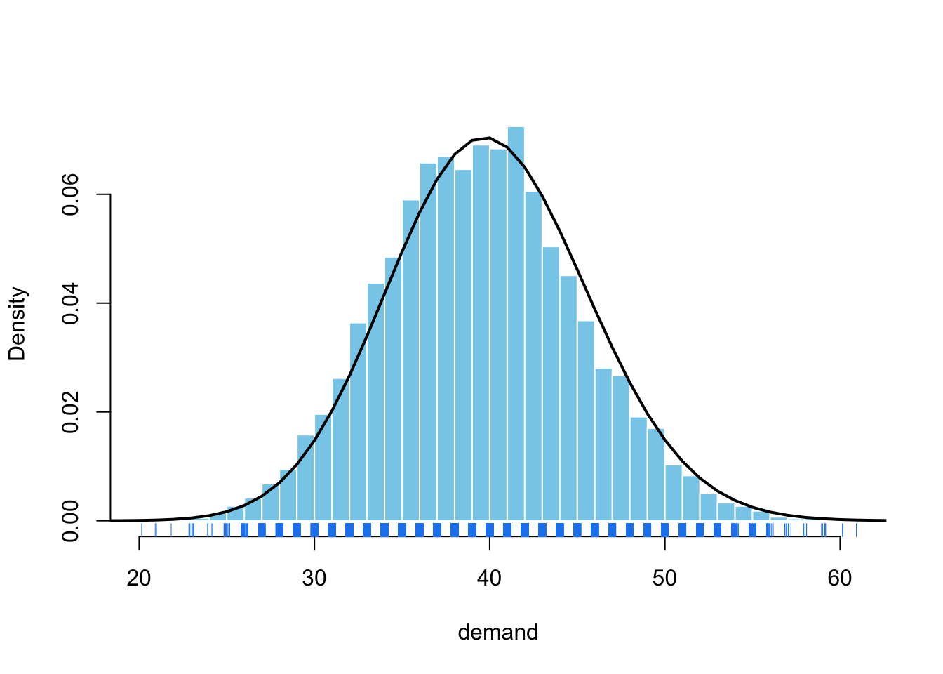
Let’s say that in our neighborhood there are 200 people walking by our shop on Mondays, and each has a 20% chance to buy, as they really love the pastries. As you can see below, the story is more complicated than just deciding to produce the average \(\mathbb{E}[D] = n \theta\).
First, notice that we can reasonably expect to sell between 30 and 50 units based on the distribution of demand. However, we need to simulate how this uncertainty translates into the distribution of profits for each quantity we might decide to produce.
set.seed(13753)

p <- 3.4; c <- 1.9; n <- 10000

sim_newsvendor <- function(p, c, qty_grid, demand) {
    df_sim <- tibble(demand = demand) |>
        mutate(nr_sim = row_number()) |>
        crossing(qty = qty_grid) |>
        mutate(
            profit = p * pmin(demand, qty) - c * qty
        )
    df_sim
}

qty_grid <- 25:70
demand <- rbinom(n, 200, 0.2)
df_sim <- sim_newsvendor(p, c, qty_grid, demand)
Show code
df_sim |> filter(qty == 47) |>
    ggplot(aes(x = profit)) +
    geom_histogram(bins = 40, fill = "skyblue", color = "white") +
    labs(x = "Profit ($)") +
theme_minimal() 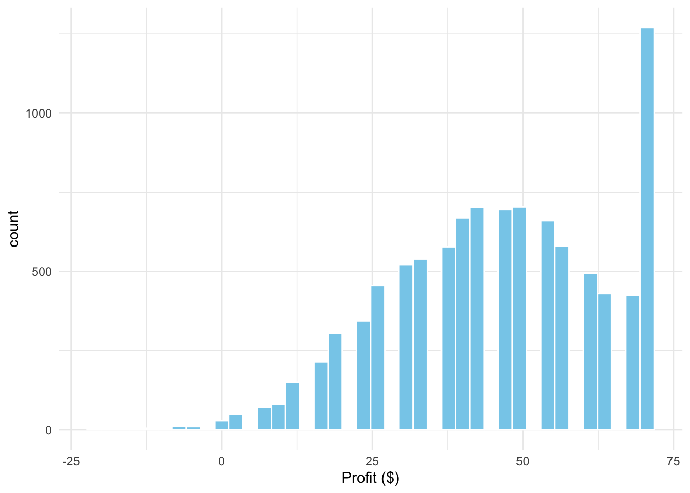
As you can see on the margin, the distribution of profits might be highly skewed. A way to represent the uncertainty in this outcome is to use highest density intervals (coda::HDPinterval()), and not the classical, symmetric confindence or credible intervals.
Another direct consequence of the uncertainty in demand and assymmetry in the cost of errors we make (underbuy vs overbuy), is that we might want a service level (availability) greater than on average. This is why we also take into consideration the 60th quantile.
Show code for aggregation and visualization
visualize_profit <- function(df_sim, hdi = 0.7, upper_q = 0.6) {
    df_sim |>
    group_by(qty) |>
    reframe(
        avg_profit = mean(profit),
        profit_upper = coda::HPDinterval(mcmc(profit), prob = hdi)[1],
        profit_lower = coda::HPDinterval(mcmc(profit), prob = hdi)[2],
        upper_profit = quantile(profit, probs = upper_q)
    ) |>
    ggplot(aes(x = qty, y = avg_profit)) +
    geom_point() +
    geom_point(aes(y = upper_profit), color = "coral") +
    geom_segment(aes(
        y = profit_lower, yend = profit_upper,
        x = qty, xend = qty
    )) +
    labs(
        x = "quantity ordered", y = "Profit ($)",
        title = "Expectation max. might not be what we want",
        subtitle = "Suggested by 70% highest density interval, not conf. int."
    ) +
    theme_minimal()
}

visualize_profit(df_sim)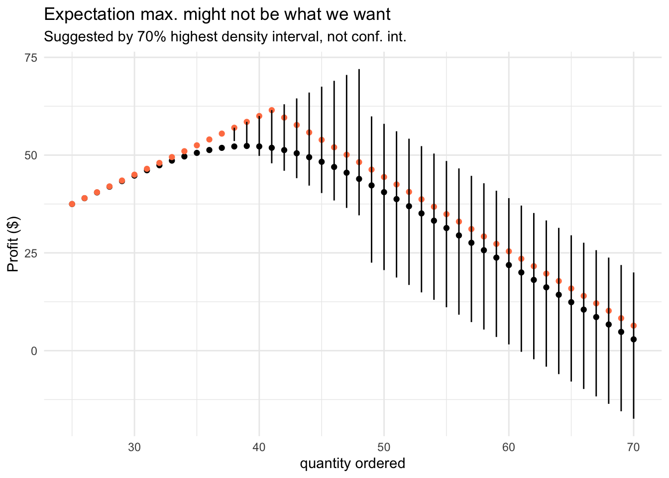
This simulation tells us that we should be very careful when optimizing for average demand. By choosing a higher service level, we will have sufficient products to fully fulfill the demand on more Mondays. It makes total sense from the perspective of customer experience and you should get used to such reasoning when making decisions under uncertainty.4 You would miss all this nuance if you’re ignoring the stochastic nature of the demand and pretend that it’s deterministic, or even worse, constant.
4 This is where other aspects inform the decision, including the firm’s risk appetite
Next, let’s investigate what happens when we deal with a “slow-moving” item, meaning, we sell a low quantity. In this case, the Poisson distribution and its generalizations might be an appropriate choice for modeling counts.
\[ D \sim Pois(\lambda = 10) \] A useful tip in practice, when dealing with slow-moving products, is that you can use the Poisson distribution as a baseline against which you can benchmark more advanced models, which often won’t do much better.
qty_grid <- 1:20
demand <- rpois(n = n, lambda = 10)
df_sim_pois <- sim_newsvendor(p, c, qty_grid, demand)

visualize_profit(df_sim_pois) 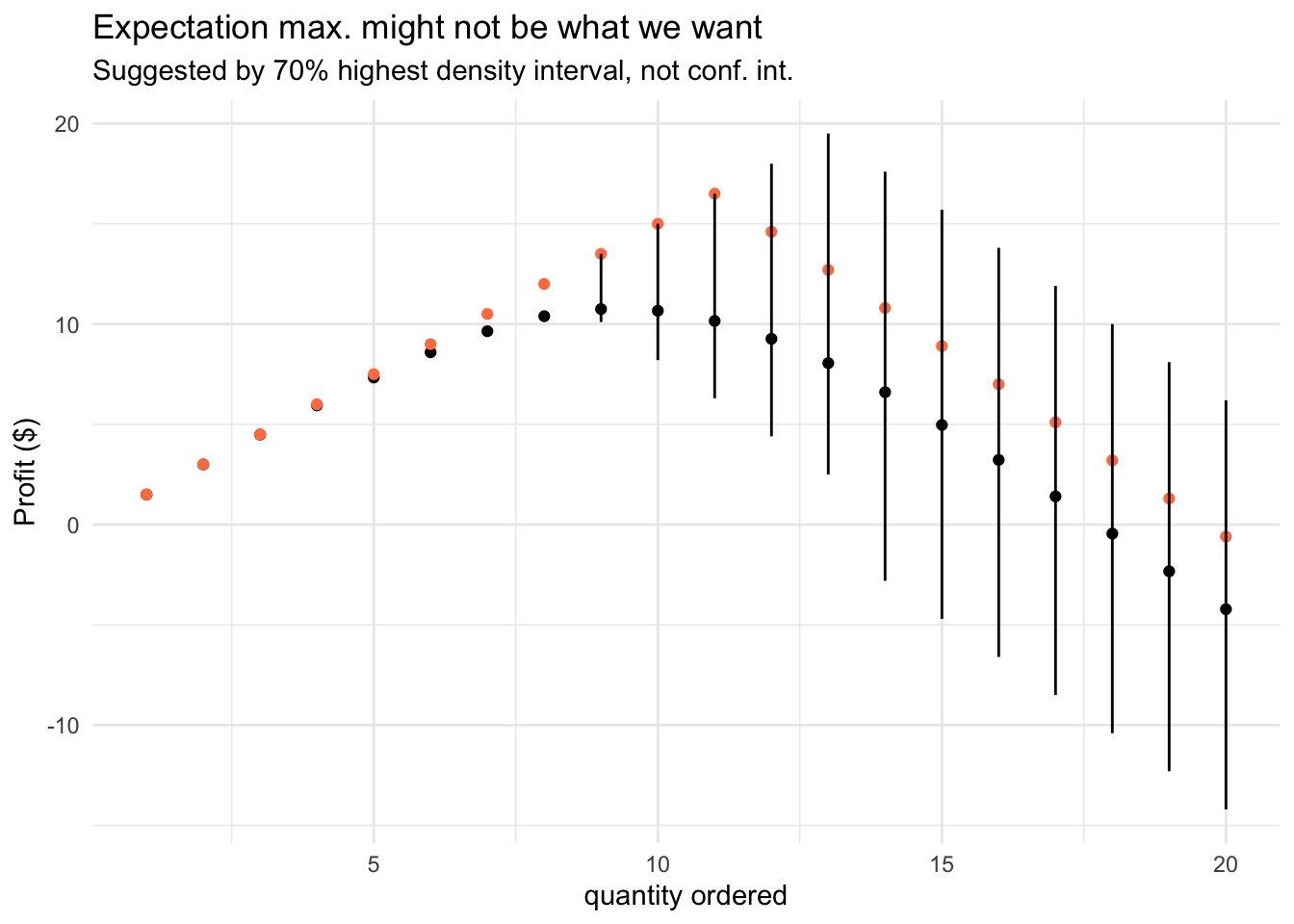
Sometimes, you have to model intermittent demand, where you will have periods in which you sell nothing. In an e-commerce or grocery store, these products might be not what we care about, but when we talk luxury items – it’s a feature, not a bug.
Once again, we can leverage the idea of a mixture model, in which we break down the demand into its occurrence and volume components. This idea was successfully used by I. Svetunkov to develop a cutting-edge time series model for forecasting intermittent demand.5
5 I. Svetunkov - “Forecasting and analytics with ADAM”, Chapter 13
\[ D \sim Bern(\theta) \cdot P(Y) \] Let’s take an example of a dish which requires expensive ingredients, like a fresh tuna steak. Here, the story is very different and we’re out of luck – it shouldn’t be surprising that we lose money in half of the days. Perisable products and intermittent demand is not a great business idea, unless there is another reason for having it.
qty_grid <- 1:20
demand <- rpois(n = n, lambda = 10) * rbinom(n = n, size = 1, prob = 0.4)
df_sim_tuna <- sim_newsvendor(p = 100, c = 30, qty_grid = qty_grid, demand = demand)

visualize_profit(df_sim_tuna) 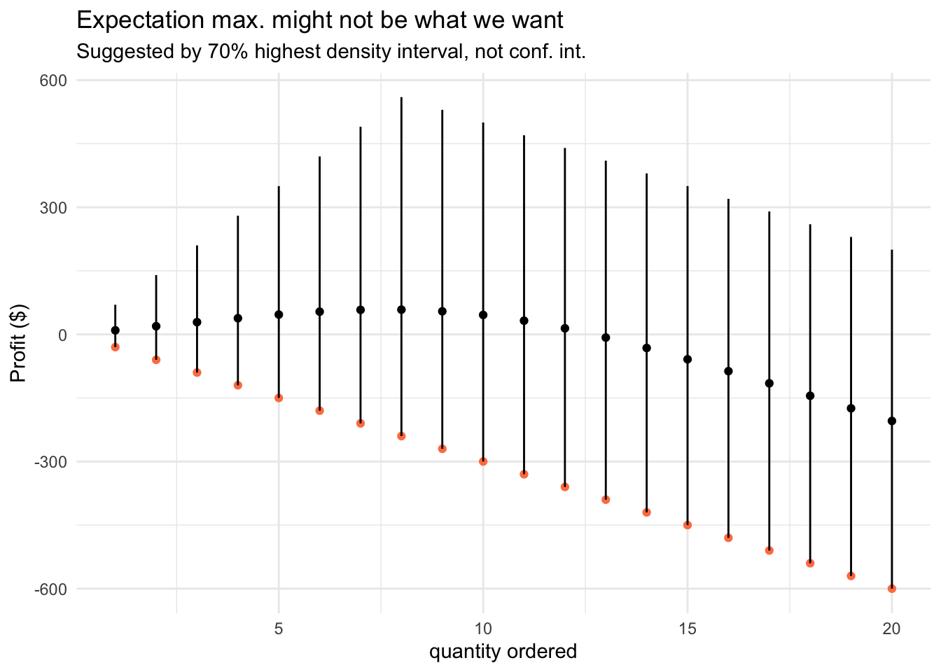
At last, we can look at fast-moving items, which sell a lot (stably) – like bread and milk in a supermarket. On the one hand we can predict the demand better, but we should also keep in mind that these products have a low gross margin.
qty_grid <- 280:320
demand <- rnorm(n = n, mean = 300, sd = 25)
df_sim_norm <- sim_newsvendor(p, c, qty_grid, demand)

visualize_profit(df_sim_norm) 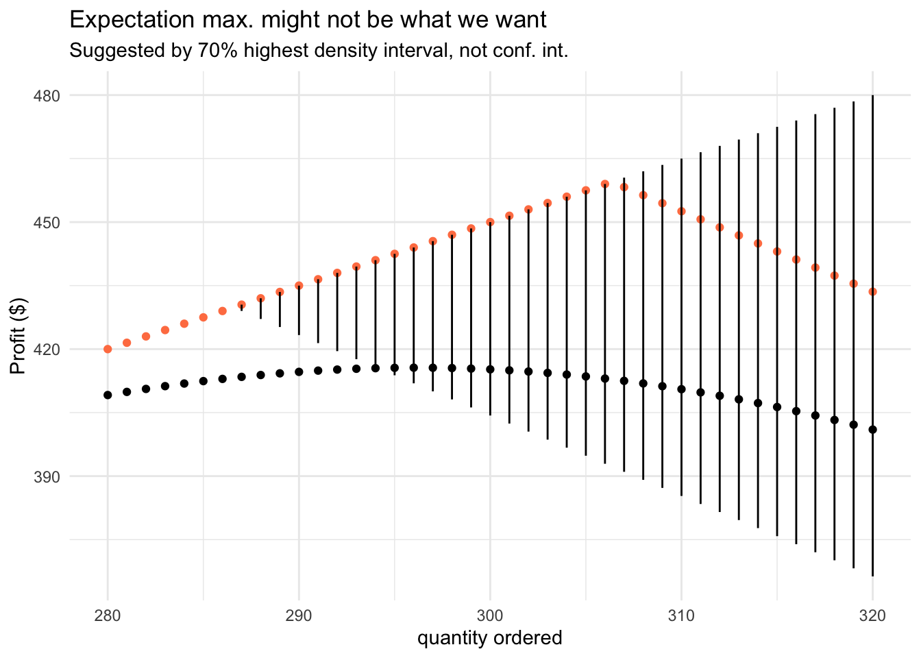
Technically, the normal distribution isn’t appropriate for modeling counts, since it is continuous and can take negative values. However, when used in the right context, with appropriate guardrails, it can be a good enough approximation in practice.
In practice, the sales data is not equivalent to demand. When building models for demand forecasting, we should be aware of the following nasty feedback loop:
- If we don’t correct for stock-outs, we’ll underestimate demand
- Which leads to lower quantities ordered and lower stocks
- Which leads to more stock-outs
- Resulting in a further underestimation of demand
Most often, we can’t know for sure how much we would sell if we had inventory. We can estimate it based on customer behavior and feedback, ignore some data points, order more than “optimal” to learn more about the demand, or build models to estimate this counterfactual.
A Poisson Detour
I often hear the following statement, especially about probability theory: “I haven’t used Poisson outside university”. By now, you’re either aware that it’s important and wonder why it didn’t come up in practice or believe it was a tedious academic exercise.
The point is not about Poisson distribution, but about probability and statistics theory in general. First, let me assure you that it is helpful in practical applications. Poisson distribution and process can be a good choice to model counts of events per unit of time and space, with a large number of “trials”, each with a small probability of success.
\[ P(X=k) = \frac{e^{−\lambda} \lambda^k}{k!}; \space k=0, 1, ... \] Poisson distribution is often a building block in more complicated models (poisson regression, gamma-poisson, GLMs), which can be used in the following applications:
- Arrivals per hour: requests in a call center, arrivals at a restaurant, website visits. We can use it for capacity planning.
- Bankrupcies filed per month, mechanical piece failures per week, engine shutdowns, work-related accidents. We can use these insights to assess risk and improve safety.
- Forecasting slow-moving items in a retail store, e.g. for clothing
- A famous example by L. Bortkiewicz: in Prussian army there were 0.70 deaths per one corps per one year caused by horse kicks. Here is the historical data and a blog post telling the story of the “Law of small numbers”.
- Number of asthma or kindey cancer related deaths
Just before you get all excited about these applications, keep in mind that every distribution has a set of assumptions that have to be met. This is where knowing the theory makes a difference.
The mathematics of newsvendor
There are more insights to be discovered than what we did in our simulation. For that, we’ll have to investigate the cost function, marginal overstock and understock costs, under discrete and continuous demand.6 We also need to look at other performance measures, like fill rate, expected leftover inventory, and in-stock probability.
6 To simplify notation, \(\mathbb{E}[max(x, 0)] = \mathbb{E}[x]^+\).
\[\begin{align} \mathcal{C}(Q) &= c_u \cdot \underbrace{ \mathbb{E}[D - Q]^+}_\text{shortage} + c_o \cdot \underbrace{ \mathbb{E}[Q - D]^+ }_\text{excess} \\ &= c_u \int_Q^\infty (D - Q) f(D) dD + c_o \int_0^Q(Q - D) f(D) dD \end{align}\]
The two terms represent total understock and overstock costs, which are convex functions of quantity. Their trade-off gives the shape of \(\mathcal{C}(Q)\) and suggests a strategy for finding the optimum.7 Before showing how to derive this result, let’s first review this important quantity called critical fractile \(\tau = c_u / (c_u + c_o)\).
7 There is a tedious and an easy, but abstract way to derive the relation for optimum
\[ Q^* = F^{-1}_D \bigg( \frac{c_u}{c_u + c_o} \bigg) \]
By plugging the critical fractile into the inverse CDF of demand, be it theoretical or empirical, we will get the optimal quantity, where the marginal cost of overage equals the marginal cost of shortages. Therefore, the optimum is determined by the asymmetric cost structure and the shape of the demand distribution.
crit_frac <- (p - c) / (p - c + c)
qty_bin <- qbinom(crit_frac, size = 200, prob = 0.2)
qty_pois <- qpois(crit_frac, lambda = 10)
qty_bin_ecdf <- quantile(rbinom(n, 200, 0.2), probs = crit_frac)
c("binomial" = qty_bin,
  "bin_ecdf" = unname(qty_bin_ecdf),
  "poisson" = qty_pois)
binomial bin_ecdf poisson
39 39 9 ecdf(rbinom(100, 200, 0.2)) |>
plot(main = "ECDF of Binom(200, 0.2)")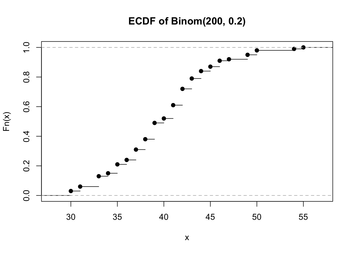
Check these results against what we obtained in our simulations. Take some time to modify the code by adding a salvage price \(s_v\) and see how does it change the optimal values.
It’s easiest to show how to arrive at the critical fractile in the case of discrete distribution of demand. The optimal point is at a place where the expected cost of ordering \(Q\) units is very close to \(Q+1\) units, i.e. the cost curve is flat – \(\mathcal{c}(Q) = \mathcal{c}(Q + 1)\).
\[ \mathcal{C}(Q) = c_o \sum_{D=0}^{Q-1} p(D) (Q - D) + c_u \sum_{D=Q}^{\infty} p(D)(D - Q) \] By using the fact that \(D - Q = 0\) when \(Q = D\), we can bring the above sums over the same range as for \(Q+1\) units.
\[\begin{align} & c_o \sum_{D=0}^{Q} p(D) (Q - D) + c_u \sum_{D=Q + 1}^{\infty} p(D)(D - Q) \\ &= c_o \sum_{D=0}^{Q} p(D) (Q + 1 - D) + c_u \sum_{D=Q+1}^{\infty} p(D)(D - Q) \end{align}\]
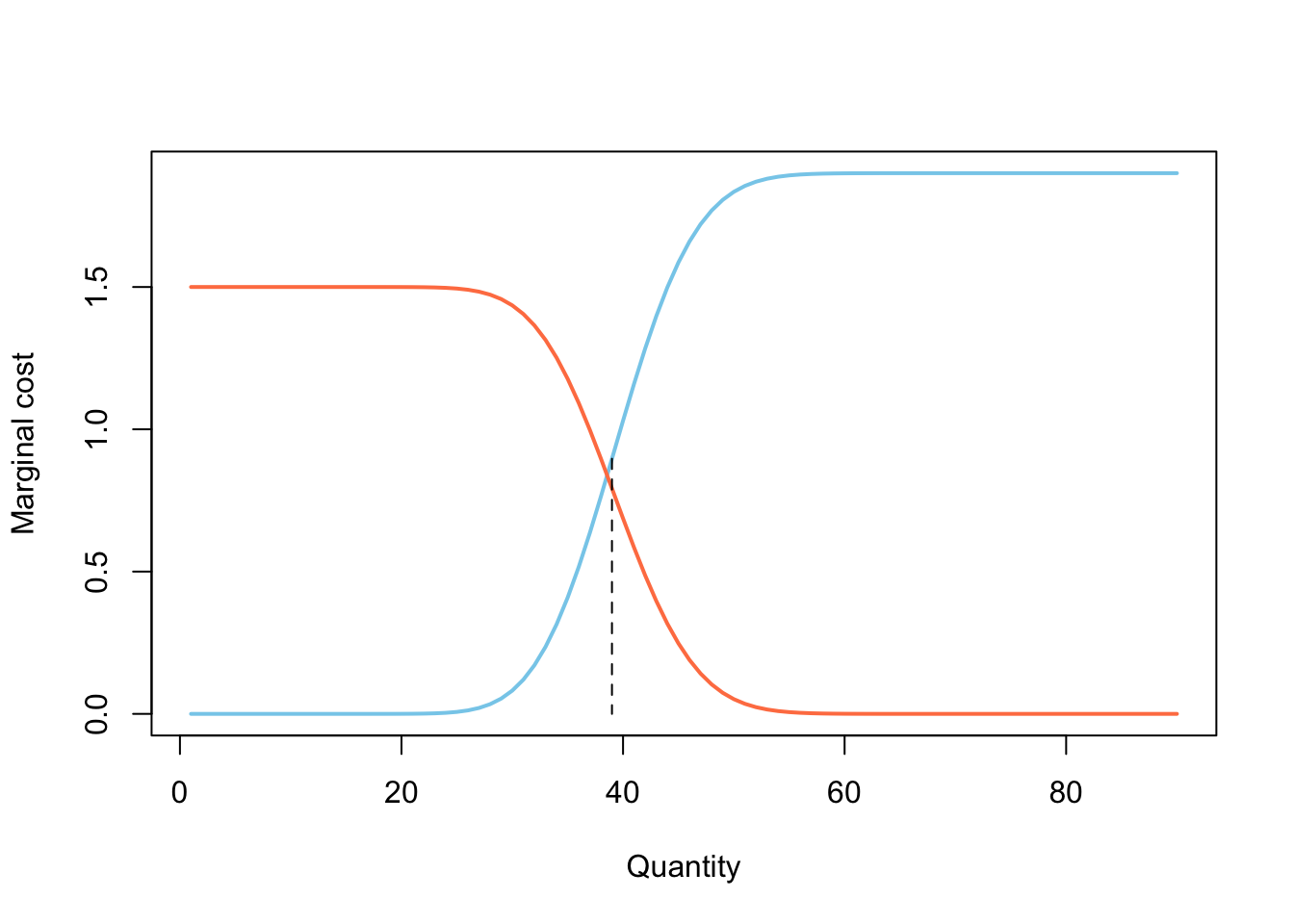
All of this mess, after grouping the appropriate terms, simplifies to the following relation. From it, you can compute the critical fractile, but also notice that we got the marginal costs for over and understocking.8
8 The optimal quantity \(Q^* = \inf \{Q | F(Q) \ge \tau \}\) is the smallest qty for which the CDF is bigger or equal than the critical value
\[ c_o \underbrace{\sum_{D = 0}^Q p(D)}_\text{F(Q)} - c_u \underbrace{\sum_{D = Q + 1}^\infty p(D)}_\text{1 - F(Q)} = 0 \]
x_grid <- 1:90
mg_cost_over <- c * pbinom(x_grid, size = 200, prob = 0.2)
mg_cost_under <- (p - c) * (1 - pbinom(x_grid, size = 200, prob = 0.2))

plot(x = x_grid, y = mg_cost_over,
     type = "l", lwd = 2, col = "skyblue",
     xlab = "Quantity", ylab = "Marginal cost", main = "")
lines(mg_cost_under, lwd = 2, col = "coral")
segments(
    x0 = qty_bin, y0 = mg_cost_over[qty_bin],
    x1 = qty_bin, y1 = 0,
    lty = "dashed"
)
There is a growing literature on the cognitive and behavioral aspects of decision-making in the newsvendor problem. First, people tend to buy less than necessary, even when the product has a big margin and critical fractile. This might be due to the fact that excess inventory is easier to measure and that information is foregrounded for the planner. When the (profit) margins are low, people generally over-buy, perhaps by putting a weight on the goodwill costs, even when it’s not the case. As you have seen from these simulations, this problem is deceptively simple – thus any heuristic or mental “calculation” can backfire.
Continuous demand
At last, in order to derive the critical fractile for the continuous distribution, we’ll need to set the first derivative of the total cost function to zero. This works out, because the function is convex – we do have an unique minimum.
\[ \mathcal{C}(Q) = c_o \int_{D=0}^Q(Q - D) f(D) dD + c_u \int_{D = Q}^\infty (D - Q) f(D) dD \]
The clearest, although tedious derivation is given by A. Hill in his 2017 paper on Newsvendor problem. For a more elegant, but abstract approach, you can check out the chapter on Stochastic Inventory Control, pg. 118 from R. Rossi’s “Inventory Analytics”.9
9 In Inventory Analytics you will also find the proof that maximizing profits and minimizing costs are equivalent in the newsvendor problem.
\[\begin{align} \mathcal{C}(Q) &= c_o Q \underbrace{\int_{D=0}^Q f(D) dD}_\text{F(Q)} - c_o \underbrace{\int_{D = 0}^Q Df(D)dD}_\text{partial expectation H(Q)} \\ &+ c_u \underbrace{\int_{D = Q}^\infty Df(D)dD}_\text{use partial expectation} - c_u Q \underbrace{\int_{D = Q}^\infty f(D)dD}_\text{1 - F(Q)} \\ \mathcal{C}(Q) &= c_o Q F(Q) - c_o H(Q) \\ & + c_u (\mu - H(Q)) - c_u Q (1 - F(Q)) \\ \end{align}\]
In the first stage, we factor out the terms and recognize where we have just a CDF of demand \(F_D(Q)\). The second term has the same form as the expectation, but doesn’t go until infinity, but only to Q. The trick is to call it a partial expectation \(H(Q)\), where \(H_D(\infty) = \mathbb{E}[D] = \mu\). Thus, the third term is just \(\mu - H(Q)\). The following is just a re-arrangement of terms which will make taking the derivative easy.
\[\begin{align} \mathcal{C}(Q) &= c_o Q F(Q) + c_u QF(Q) \\ &- c_o H(Q) - c_u H(Q) \\ & + c_u \mu - c_u Q \\ \mathcal{C}(Q) & = (c_u + c_o)(QF(Q) - H(Q)) + c_u (\mu - Q) \end{align}\]
Now we’re ready to take the derivative and set it to zero. The only thing you have to remember is that \(F'(Q) = f(Q)\) and \(H'(Q) = Q f(Q)\) by Leibniz’s rule.10
10 These details are completely optional and outside the scope of the course
\[\begin{align} \mathcal{C}'(Q) &= (c_u + c_o)[QF'(Q) + F(Q) - H'(Q)] - c_u \\ &= (c_u + c_o)[Qf(Q) + F(Q) - Qf(Q)] - c_u \\ 0 &= (c_u + c_o)F(Q) - c_u \\ F(Q) &= \frac{c_u}{c_u + c_o} \end{align}\]
Finally, we’ve proven the relation for the critical fractile and can leverage the marginal overage and underage costs.
\[ \mathcal{C}'(Q) = c_oF(Q) - c_u [1- F(Q)] \]
Homework
Modify the code in the course to take into account the salvage value \(s_v\) and interpret how the results of the simulations change. Experiment on different situations where the profit margins are low (like in a grocery store) or quite high. Try out demand with high and low uncertainty, asymmetric and long-tailed distributions.
- Read the paper by A. Hill and note the other metrics that we can look at besides profits and costs (Appendix 3).
- Read the paper by M. Koschat, N. Kunz - “Newsvendors tackle the newsvendor problem”, 2003